The following objects are masked from 'package:dplyr':

    between, lag, lead
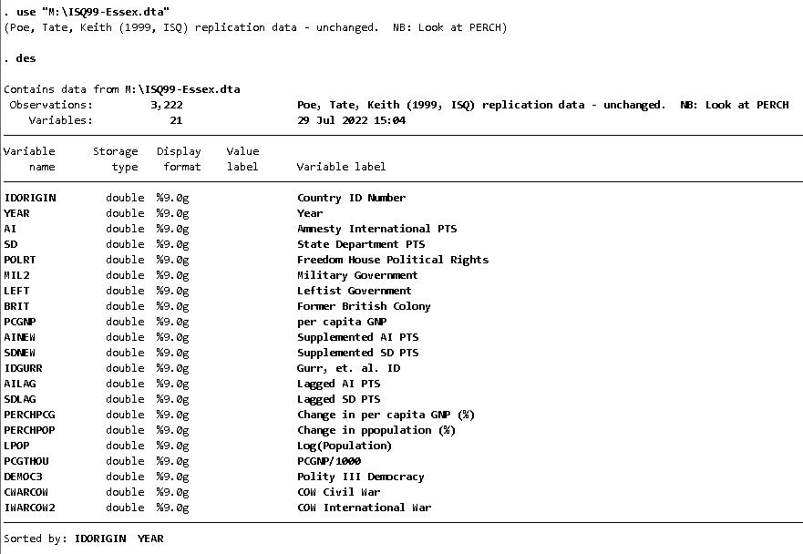
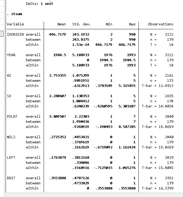
source(url("https://raw.githubusercontent.com/robertwwalker/DADMStuff/master/xtsum.R"))# Be careful with the ID variable, the safest is to make it factor; this can go wildly wrongxtsum(IDORIGIN~., data=HR.Data) %>%kable() %>%scroll_box(width="80%", height="50%")
Note: Using an external vector in selections is ambiguous.
ℹ Use `all_of(unit)` instead of `unit` to silence this message.
ℹ See <https://tidyselect.r-lib.org/reference/faq-external-vector.html>.
This message is displayed once per session.
O.mean
O.sd
O.min
O.max
O.SumSQ
O.N
B.mean
B.sd
B.min
B.max
B.Units
B.t.bar
W.sd
W.min
W.max
W.SumSQ
Within.Ovr.Ratio
YEAR
1984.5
5.189
1976
1993
86725.5
3222
1984.5
0
1984.5
1984.5
179
18
5.189
-8.5
8.5
86725.5
1
AI
2.753
1.075
1
5
2497.538
2161
2.498
0.989
1
5
173
12.491
0.631
-2.375
2.5625
860.822
0.345
SD
2.241
1.13
1
5
3365.455
2635
2.241
1.004
1
5
178
14.803
0.624
-2.666667
3.0625
1025.695
0.305
POLRT
3.81
2.223
1
7
14029.94
2840
3.78
1.99
1
7
179
15.866
0.925
-4
4.777778
2428.552
0.173
MIL2
0.273
0.445
0
1
563.058
2840
0.24
0.377
0
1
179
15.866
0.216
-0.9444444
0.8888889
132.778
0.236
LEFT
0.176
0.381
0
1
410.983
2829
0.157
0.334
0
1
179
15.804
0.157
-0.8888889
0.8888889
69.611
0.169
BRIT
0.355
0.479
0
1
671.685
2932
0.335
0.473
0
1
179
16.38
0
0
0
0
0
PCGNP
3591.651
5698.355
52
36670
90205144379
2779
3449.178
5049.297
112.2222
22653.89
173
16.064
2278.412
-12303.33
16961.67
14421042273
0.16
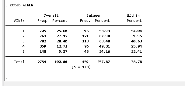
AINEW
2.443
1.156
1
5
3677.663
2754
2.379
1.012
1
5
178
15.472
0.622
-2.388889
2.944444
1064.102
0.289
SDNEW
2.262
1.137
1
5
3556.241
2754
2.253
1.006
1
5
178
15.472
0.631
-2.588235
3
1096.442
0.308
IDGURR
455.771
246.52
2
990
195747185
3222
455.771
247.173
2
990
179
18
0
0
0
0
0
AILAG
2.45
1.148
1
5
3396.045
2578
2.402
1.039
1
5
177
14.565
0.609
-2.411765
3
955.37
0.281
SDLAG
2.247
1.116
1
5
3207.603
2578
2.236
0.991
1
5
177
14.565
0.608
-2.5
3.058824
952.174
0.297
PERCHPCG
4.614
13.221
-95.5
128.57
454983.6
2604
3.325
6.893
-36.21333
15.03765
168
15.5
12.393
-92.50235
114.8882
399763
0.879
PERCHPOP
2.193
4.042
-48.45
126.01
47846.75
2929
2.842
9.443
-2.126471
126.01
176
16.642
3.018
-48.12235
80.69765
26663.59
0.557
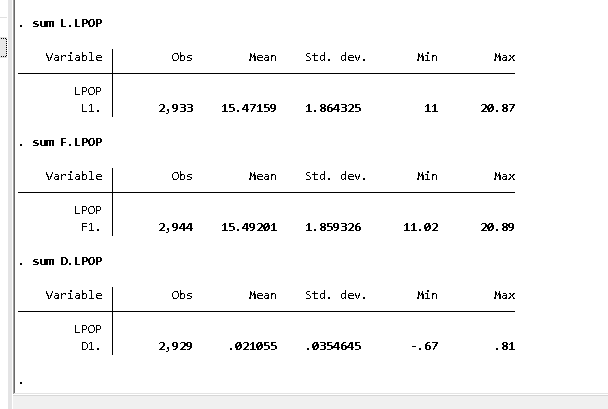
LPOP
15.482
1.863
11
20.89
10784.05
3107
15.488
1.844
11.09056
20.76889
177
17.554
0.129
-0.7288889
0.7311111
51.883
0.005
PCGTHOU
3.592
5.698
0.05
36.67
90204.45
2779
3.449
5.049
0.1122222
22.65389
173
16.064
2.278
-12.30333
16.96167
14420.95
0.16
DEMOC3
3.682
4.358
0
10
46107
2429
3.774
3.96
0
10
155
15.671
1.726
-7.277778
7.941176
7229.815
0.157
CWARCOW
0.092
0.289
0
1
235.17
2815
0.095
0.245
0
1
179
15.726
0.175
-0.8888889
0.9444444
85.693
0.364
IWARCOW2
0.086
0.281
0
1
223.879
2842
0.092
0.227
0
1
179
15.877
0.19
-0.8888889
0.9444444
102.992
0.46
The Core Idea
In R, this is an essential group_by calculation in the tidyverse. The between data are a summary table with units constituting the rows. The within data is the overall data with group means subtracted.
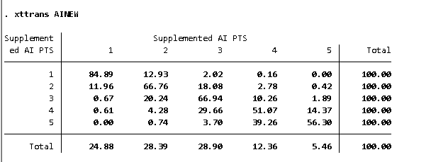
I want to rely on the dplyr version of lag so I am explicit here. Take the data, group it by id, calculate the lag, ungroup them, and create a table. I prefer to keep this explicit with order_by. The janitor library provides tabyl and it is explicit among missing values.
 I want to rely on the