Day 2: Time Series, Stationarity, and ARIMA Models

time series
code
analysis
Author

Robert W. Walker

Published

August 9, 2022

Slides

Simulating ARIMA processes

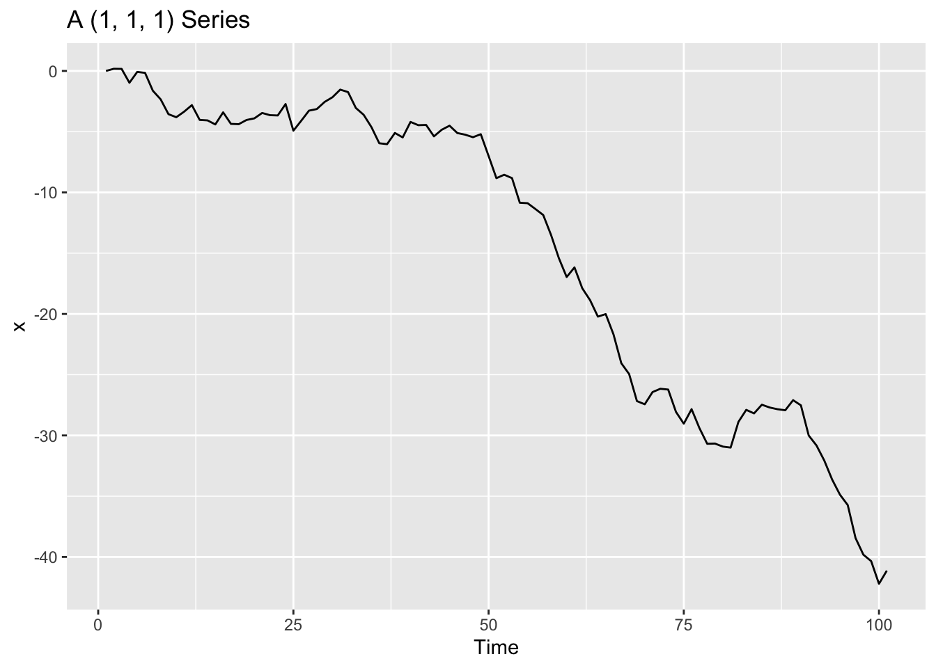
We want to simulate data under an ARIMA (p, d, q) model. arima.sim wants inputs as a list where the expected length of the ar and ma vectors that will hold the actual values of the ar and ma parameters. Here, I ask for a series that is I(1) with a first-order ar=0.1 and a first-order ma=-0.5. Let me start by generating it and plotting the time series.

library(fpp3)
── Attaching packages ──────────────────────────────────────────── fpp3 0.4.0 ──
✔ tibble      3.1.8     ✔ tsibble     1.1.1
✔ dplyr       1.0.9     ✔ tsibbledata 0.4.0
✔ tidyr       1.2.0     ✔ feasts      0.2.2
✔ lubridate   1.8.0     ✔ fable       0.3.1
✔ ggplot2     3.3.6     
── Conflicts ───────────────────────────────────────────────── fpp3_conflicts ──
✖ lubridate::date()    masks base::date()
✖ dplyr::filter()      masks stats::filter()
✖ tsibble::intersect() masks base::intersect()
✖ tsibble::interval()  masks lubridate::interval()
✖ dplyr::lag()         masks stats::lag()
✖ tsibble::setdiff()   masks base::setdiff()
✖ tsibble::union()     masks base::union()
n <- 100
my.data <- data.frame(
  x=arima.sim(n = n, 
              model=list(order = c(1, 1, 1), ar=c(0.7), ma=c(-0.5)), n.start=20), 
  dtime = seq(1,n+1))
library(magrittr)

Attaching package: 'magrittr'
The following object is masked from 'package:tidyr':

    extract
my.data %<>% as_tsibble(index=dtime) 
my.data %>% autoplot() + labs(title="A (1, 1, 1) Series", x="Time")
Plot variable not specified, automatically selected `.vars = x`

Now I want to display the ACF and PACF in levels.

library(patchwork)
{my.data %>% ACF(x, lag_max=20) %>% 
    autoplot() } + 
  {my.data %>% PACF(x, lag_max=20) %>% 
      autoplot() }

Finally, let me display the ACF and PACF with differenced data.

{my.data %>% ACF(diff(x), lag_max=20) %>% 
    autoplot() } + 
  {my.data %>% PACF(diff(x), lag_max=20) %>% 
      autoplot() }

Nonsense Regressions of I(1) Series

An Example of Time Series Troubles

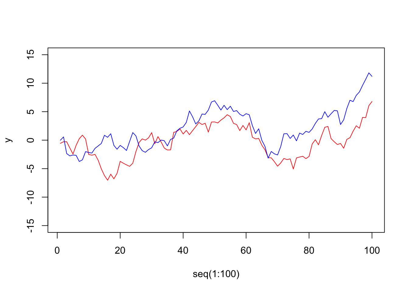
Let me do this with a relatively simple regression. Two variables:

\[ y = \alpha + \beta x + \epsilon \]

Both are generated randomly. Here’s a basic plot.

y <- cumsum(rnorm(100))
x <- cumsum(rnorm(100))
plot(x=seq(1:100), y=y, type="l", col="red", ylim=c(-15,15))
lines(x=seq(1:100), y=x, col="blue")

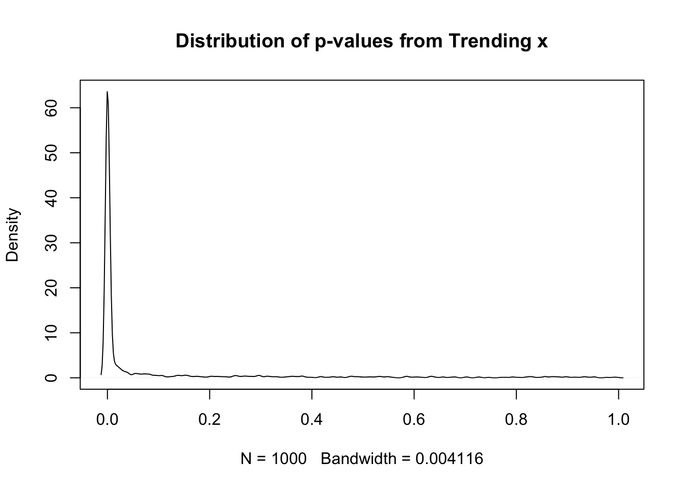
Each time series contains 100 observations. Because both x and y are random, the slopes should be 0, 95% of the time with 95% confidence because there is no underlying relationship. In practice, let’s look at the distribution of p-values for the probability of no relationship.

SR <- function(n) {
  Results <- NULL
  for(i in 1:n) {
y <- cumsum(rnorm(100))
x <- cumsum(rnorm(100))
Result <- summary(lm(y~x))$coefficients[2,4]
Results <- append(Result,Results)
  }
  Results
}

I replicate the process of random x and random y 1000 times and show the p-values below. Because they are random, approximately 95% should be greater than 0.05.

Res1 <- SR(1000)
plot(density(Res1), main="Distribution of p-values from Trending x")

In practice,

table(Res1 > 0.05)

FALSE  TRUE 
  779   221 

The above table should show about 950 TRUE and 50 FALSE but because each is trended and they share variation from trend, the actual frequency of rejecting the claim of no relationship is far more common than 5%.

ARIMA Models with Government Popularity

library(fpp3)
library(haven)
br7983 <- read_dta(url("https://github.com/robertwwalker/Essex-Data/raw/main/br7983.dta")) %>% 
  mutate(month = as.character(month)) %>% 
  mutate(month = paste0("19",month, sep="")) %>% 
  mutate(date = yearmonth(month, format="%Y%m"))
br7983 <- br7983 %>% as_tsibble(index=date) 
br7983 %>% autoplot(govpopl) + hrbrthemes::theme_ipsum() + labs(y="logged Government Popularity")

Time Series Features

br7983 %>% gg_tsdisplay(govpopl, plot_type = "partial")

library(haven)
# To install TSA, it works in three steps.
# Link to package
# https://cran.r-project.org/web/packages/TSA/index.html
# The archive for the package is:
# https://cran.r-project.org/src/contrib/Archive/TSA/
# I grabbed the most recent one.
# Then I used the RStudio: Tools > Install Packages > From a local archive
# And installed it.
# It had dependency chains to fix.
# Those can be fixed with
# install.packages(c("leaps", "locfit", "mgcv"))
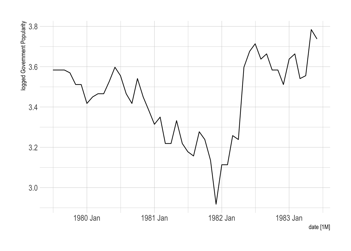
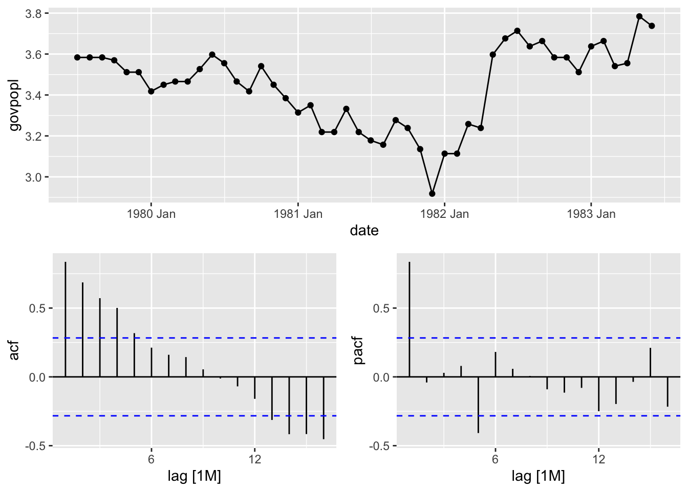
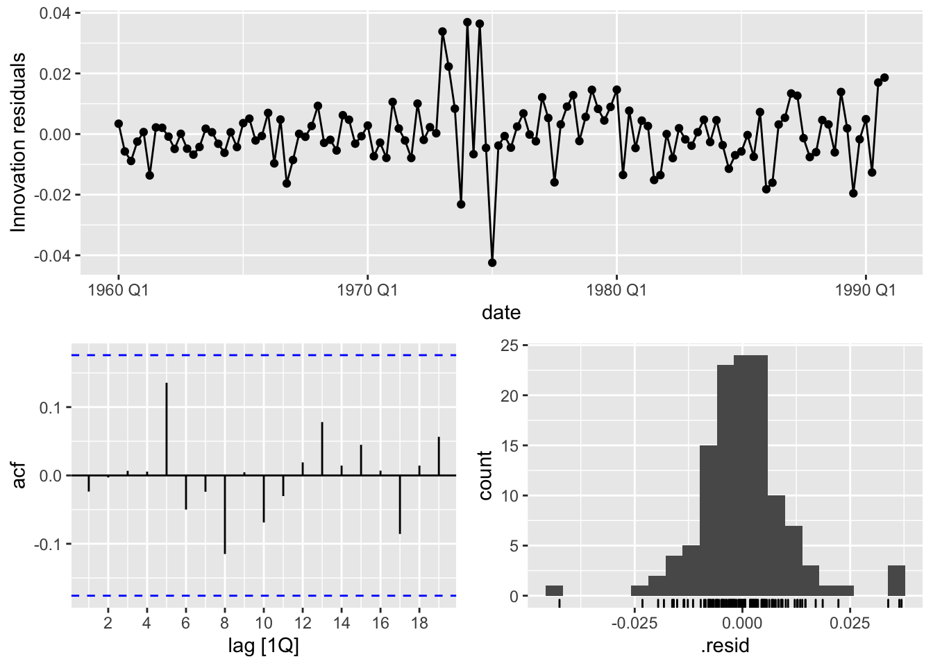
library(TSA)
# Replicating the abrupt permanent in April
arimax(br7983$govpopld, seasonal = list(order = c(0, 0, 1), period = 4), xreg=br7983$flandd)

Call:
arimax(x = br7983$govpopld, seasonal = list(order = c(0, 0, 1), period = 4), 
    xreg = br7983$flandd)

Coefficients:
        sma1  intercept    xreg
      0.3430     0.0015  0.0687
s.e.  0.1347     0.0184  0.0950

sigma^2 estimated as 0.009071:  log likelihood = 43.57,  aic = -81.15
# Replicating the abrupt permanent in May
arimax(br7983$govpopld, seasonal = list(order = c(0, 0, 1), period = 4), xreg=br7983$flanddlag1)

Call:
arimax(x = br7983$govpopld, seasonal = list(order = c(0, 0, 1), period = 4), 
    xreg = br7983$flanddlag1)

Coefficients:
        sma1  intercept    xreg
      0.2668    -0.0033  0.3124
s.e.  0.1310     0.0153  0.0842

sigma^2 estimated as 0.007019:  log likelihood = 49.7,  aic = -93.41
# Replicating the gradual permanent April
arimax(br7983$govpopld, seasonal = list(order = c(0, 0, 1), period = 4), xtransf = br7983$flandd, transfer = list(c(1,0)))

Call:
arimax(x = br7983$govpopld, seasonal = list(order = c(0, 0, 1), period = 4), 
    xtransf = br7983$flandd, transfer = list(c(1, 0)))

Coefficients:
        sma1  intercept  T1-AR1  T1-MA0
      0.3930    -0.0080  0.6479  0.1885
s.e.  0.1251     0.0185  0.1528  0.0718

sigma^2 estimated as 0.007946:  log likelihood = 46.6,  aic = -85.2
# Replicating the gradual permanent May
# Does not work; degrees of freedom?
# arimax(br7983$govpopld, seasonal = list(order = c(0, 0, 1), period = 4), xtransf = br7983$flanddlag1, transfer = list(c(1,0)))
# Falklands - gradual temporary (pulse decay) effect - May 1982
# Does not work; degrees of freedom?
# arimax(br7983$govpopld, seasonal = list(order = c(0, 0, 1), period = 4), xtransf = br7983$flanddlag1, transfer = list(c(1,1)))
# These are fairly demanding [of the data] models.
arimax(br7983$govpopld, seasonal = list(order = c(0, 0, 1), period = 4), xtransf = br7983$flandd, transfer = list(c(1,0)))

Call:
arimax(x = br7983$govpopld, seasonal = list(order = c(0, 0, 1), period = 4), 
    xtransf = br7983$flandd, transfer = list(c(1, 0)))

Coefficients:
        sma1  intercept  T1-AR1  T1-MA0
      0.3930    -0.0080  0.6479  0.1885
s.e.  0.1251     0.0185  0.1528  0.0718

sigma^2 estimated as 0.007946:  log likelihood = 46.6,  aic = -85.2

ARIMA

Stata covers this in the following link.

wpi1 <- read_stata(url("http://www.stata-press.com/data/r12/wpi1.dta"))
wpi1$date <- yearquarter(wpi1$t, fiscal_start = 1)-40
load(url("https://github.com/robertwwalker/Essex-Data/raw/main/wpi1.RData"))
wpi1 %>% as_tsibble(index=date) %>% gg_tsdisplay(ln_wpi, plot_type = "partial") + labs(title="Log WPI")

Stata

arima wpi, arima(1,1,1)

R

wpi1 %>% as_tsibble(index=date) %>% 
  model(arima = ARIMA(wpi ~ 1 + pdq(1,1,1) + PDQ(0,0,0))) %>% 
  report()
Series: wpi 
Model: ARIMA(1,1,1) w/ drift 

Coefficients:
         ar1      ma1  constant
      0.8742  -0.4120    0.0943
s.e.  0.0637   0.1221    0.0367

sigma^2 estimated as 0.5388:  log likelihood=-135.35
AIC=278.7   AICc=279.04   BIC=289.95

The help for ARIMA explains the alternative parameterization.

# Using stats::arima
arima(diff(wpi1$wpi), order=c(1,0,1), include.mean = TRUE)

Call:
arima(x = diff(wpi1$wpi), order = c(1, 0, 1), include.mean = TRUE)

Coefficients:
         ar1      ma1  intercept
      0.8742  -0.4120     0.7499
s.e.  0.0637   0.1221     0.2921

sigma^2 estimated as 0.5257:  log likelihood = -135.35,  aic = 276.7

Seasonal

arima D.ln_wpi, ar(1) ma(1 4)
wpi1 %>% as_tsibble(index=date) %>% 
  model(arima = ARIMA(ln_wpi ~ 1 + pdq(1,1,1) + PDQ(0,0,1))) %>% 
  report()
Series: ln_wpi 
Model: ARIMA(1,1,1)(0,0,1)[4] w/ drift 

Coefficients:
         ar1      ma1    sma1  constant
      0.8289  -0.4252  0.2403    0.0019
s.e.  0.0854   0.1374  0.0959    0.0007

sigma^2 estimated as 0.0001144:  log likelihood=385.27
AIC=-760.53   AICc=-760.02   BIC=-746.47

There are also bits about seasonal arima – sarima – and arimax but Stata is fundamentally limited here.

wpi1 %>% as_tsibble(index=date) %>% 
  model(arima = ARIMA(ln_wpi ~ 1 + pdq(1,1,1) + PDQ(0,0,1))) %>% 
  gg_tsresiduals()

That works.