Day 3: Dynamic Linear, ADL Models, and VARs

time series
code
analysis
Author

Robert W. Walker

Published

August 10, 2022

Slides

Dynamic Regression

Regression techniques can be reexamined through the lens of dynamic linear models and systems of linear equations. Whether autoregressive distributed lag models or VAR systems and structural time series, regression approaches to time series almost inevitably culminate in thinking about causation as conceived by Clive Granger – Granger causality.

Today we cover chapters 3 and 4 in TSASS spanning dynamic regression models and dynamic systems. We will start with dynamic regression models by detailing how they are specified and interpreted with distributed lag and autoregressive distributed lag [ADL] models. We also examine the crucial issue of consistency before turning to structural time series models for multiple equations and their counterparts – VARs.

VARs

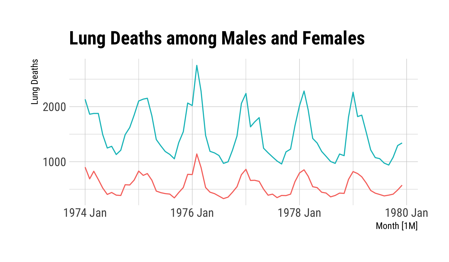
We will start with some data on lung deaths from Australia.

library(forecast)
mdeaths
fdeaths
save(mdeaths, fdeaths, file = "./img/LungDeaths.RData")
use "https://github.com/robertwwalker/Essex-Data/raw/main/Lung-Deaths.dta"
library(hrbrthemes); library(fpp3)
load(url("https://github.com/robertwwalker/Essex-Data/raw/main/LungDeaths.RData"))
Males <- mdeaths; Females <- fdeaths
Lung.Deaths <- cbind(Males, Females) %>% as_tsibble()
Lung.Deaths %>% autoplot() + theme_ipsum_rc() + labs(y="Lung Deaths", x="Month [1M]", title="Lung Deaths among Males and Females") + guides(color="none")

lung_deaths <- cbind(mdeaths, fdeaths) %>%
  as_tsibble(pivot_longer = FALSE)
lung_deaths <- cbind(mdeaths, fdeaths) %>%
  as_tsibble(pivot_longer = FALSE)
fit <- lung_deaths %>%
  model(VAR(vars(mdeaths, fdeaths) ~ AR(3)))
report(fit)
Series: mdeaths, fdeaths 
Model: VAR(3) w/ mean 

Coefficients for mdeaths:
      lag(mdeaths,1)  lag(fdeaths,1)  lag(mdeaths,2)  lag(fdeaths,2)
              0.6675          0.8074          0.3677         -1.4540
s.e.          0.3550          0.8347          0.3525          0.8088
      lag(mdeaths,3)  lag(fdeaths,3)  constant
              0.2606         -1.1214  538.7817
s.e.          0.3424          0.8143  137.1047

Coefficients for fdeaths:
      lag(mdeaths,1)  lag(fdeaths,1)  lag(mdeaths,2)  lag(fdeaths,2)
              0.2138          0.4563          0.0937         -0.3984
s.e.          0.1460          0.3434          0.1450          0.3328
      lag(mdeaths,3)  lag(fdeaths,3)  constant
              0.0250          -0.315  202.0027
s.e.          0.1409           0.335   56.4065

Residual covariance matrix:
         mdeaths  fdeaths
mdeaths 58985.95 22747.94
fdeaths 22747.94  9983.95

log likelihood = -812.35
AIC = 1660.69   AICc = 1674.37  BIC = 1700.9
var mdeaths fdeaths, lags(1 2 3)  
fit2 <- lung_deaths %>%
  model(VAR(vars(mdeaths, fdeaths) ~ AR(2)))
report(fit2)
Series: mdeaths, fdeaths 
Model: VAR(2) w/ mean 

Coefficients for mdeaths:
      lag(mdeaths,1)  lag(fdeaths,1)  lag(mdeaths,2)  lag(fdeaths,2)  constant
              0.9610          0.3340          0.1149         -1.3379  443.8492
s.e.          0.3409          0.8252          0.3410          0.7922  124.4608

Coefficients for fdeaths:
      lag(mdeaths,1)  lag(fdeaths,1)  lag(mdeaths,2)  lag(fdeaths,2)  constant
              0.3391          0.2617         -0.0601         -0.2691  145.0546
s.e.          0.1450          0.3510          0.1450          0.3369   52.9324

Residual covariance matrix:
         mdeaths  fdeaths
mdeaths 62599.51 24942.79
fdeaths 24942.79 11322.70

log likelihood = -833.17
AIC = 1694.35   AICc = 1701.98  BIC = 1725.83
var mdeaths fdeaths, lags(1 2)  

Granger causation wants a non-tidy format. I will use the conventional VAR syntax from vars that wants the collection of endogenous variables as inputs by themselves in a matrix form. We can also specify exogenous variable for such systems with their data matrix in the argument exogen=....

library(bruceR)

bruceR (version 0.8.8)
BRoadly Useful Convenient and Efficient R functions

Packages also loaded:
√ dplyr         √ emmeans       √ ggplot2
√ tidyr         √ effectsize    √ ggtext
√ stringr       √ performance   √ cowplot
√ forcats       √ lmerTest      √ see
√ data.table

Main functions of `bruceR`:
cc()            Describe()  TTEST()
add()           Freq()      MANOVA()
.mean()         Corr()      EMMEANS()
set.wd()        Alpha()     PROCESS()
import()        EFA()       model_summary()
print_table()   CFA()       lavaan_summary()

https://psychbruce.github.io/bruceR/
Varmf <- vars::VAR(lung_deaths[,c("mdeaths","fdeaths")], p=3, type="const")
granger_causality(Varmf)

Granger Causality Test (Multivariate)

F test and Wald χ² test based on VAR(3) model:
────────────────────────────────────────────────────────────────
                          F df1 df2     p     Chisq df     p    
────────────────────────────────────────────────────────────────
 ------------------                                             
 mdeaths <= fdeaths    1.93   3  62  .134      5.80  3  .122    
 mdeaths <= ALL        1.93   3  62  .134      5.80  3  .122    
 ------------------                                             
 fdeaths <= mdeaths    1.20   3  62  .316      3.61  3  .307    
 fdeaths <= ALL        1.20   3  62  .316      3.61  3  .307    
────────────────────────────────────────────────────────────────
vargranger
fit %>%
  fabletools::forecast(h=12) %>%
  autoplot(lung_deaths)

Female

lung_deaths %>%
model(VAR(vars(mdeaths, fdeaths) ~ AR(3))) %>%
  residuals() %>% 
  pivot_longer(., cols = c(mdeaths,fdeaths)) %>% 
  filter(name=="fdeaths") %>% 
  as_tsibble(index=index) %>% 
  gg_tsdisplay(plot_type = "partial") + labs(title="Female residuals")

Male

lung_deaths %>%
model(VAR(vars(mdeaths, fdeaths) ~ AR(3))) %>%
  residuals() %>% 
  pivot_longer(., cols = c(mdeaths,fdeaths)) %>% 
  filter(name=="mdeaths") %>% 
  as_tsibble(index=index) %>% 
  gg_tsdisplay(plot_type = "partial") + labs(title="Male residuals")

Easy Impulse Response

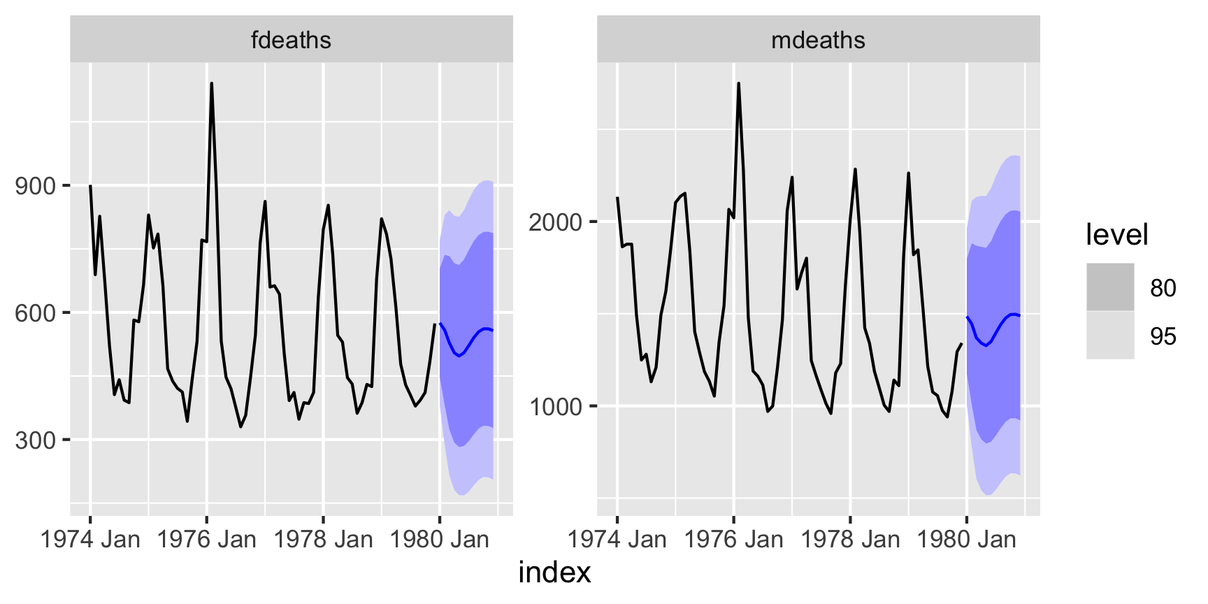
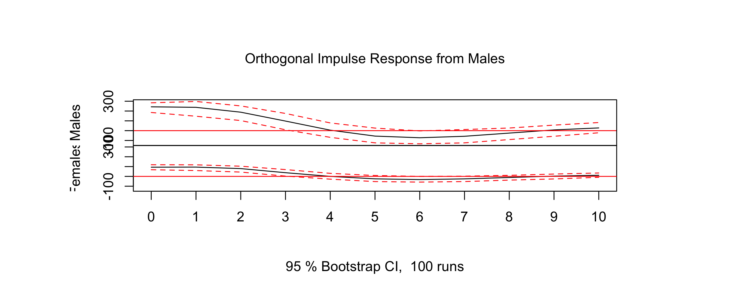
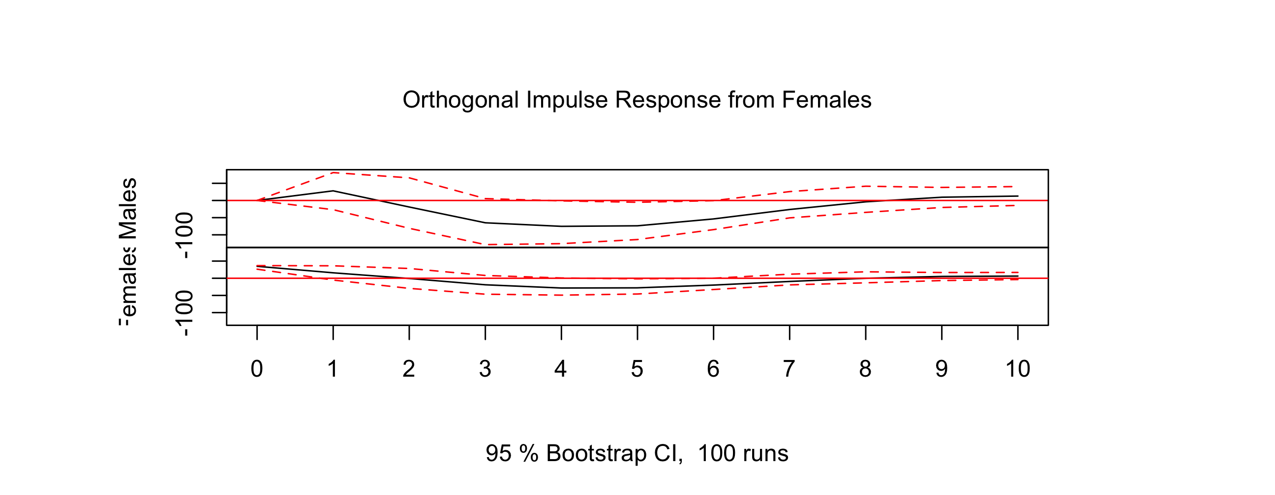
What happens if I shock one of the series; how does it work through the system?

The idea behind an impulse-response is core to counterfactual analysis with time series. What does our future world look like and what predictions arise from it and the model we have deployed?

Whether VARs or dynamic linear models or ADL models, these are key to interpreting a model in the real world.

Males

irf set "M:\t1.irf"
irf create irf1, order( mdeaths fdeaths)
irf graph irf
VARMF <- cbind(Males,Females)
mod1 <- vars::VAR(VARMF, p=3, type="const")
plot(vars::irf(mod1, boot=TRUE, impulse="Males"))

Females

irf set "M:\tF.irf"
irf create Female, order( fdeaths mdeaths)
irf graph irf
plot(vars::irf(mod1, boot=TRUE, impulse="Females"))