use "https://github.com/robertwwalker/Essex-Data/raw/main/ISQ99-Essex.dta"
xtset
drop if AINEW==.
xtset
* Give consideration to what we should do about the Lagged DV
drop if AILAG==.
* A note about long versus flong
mi set flong
* Note that it adds some variables; what are they?
mi describe
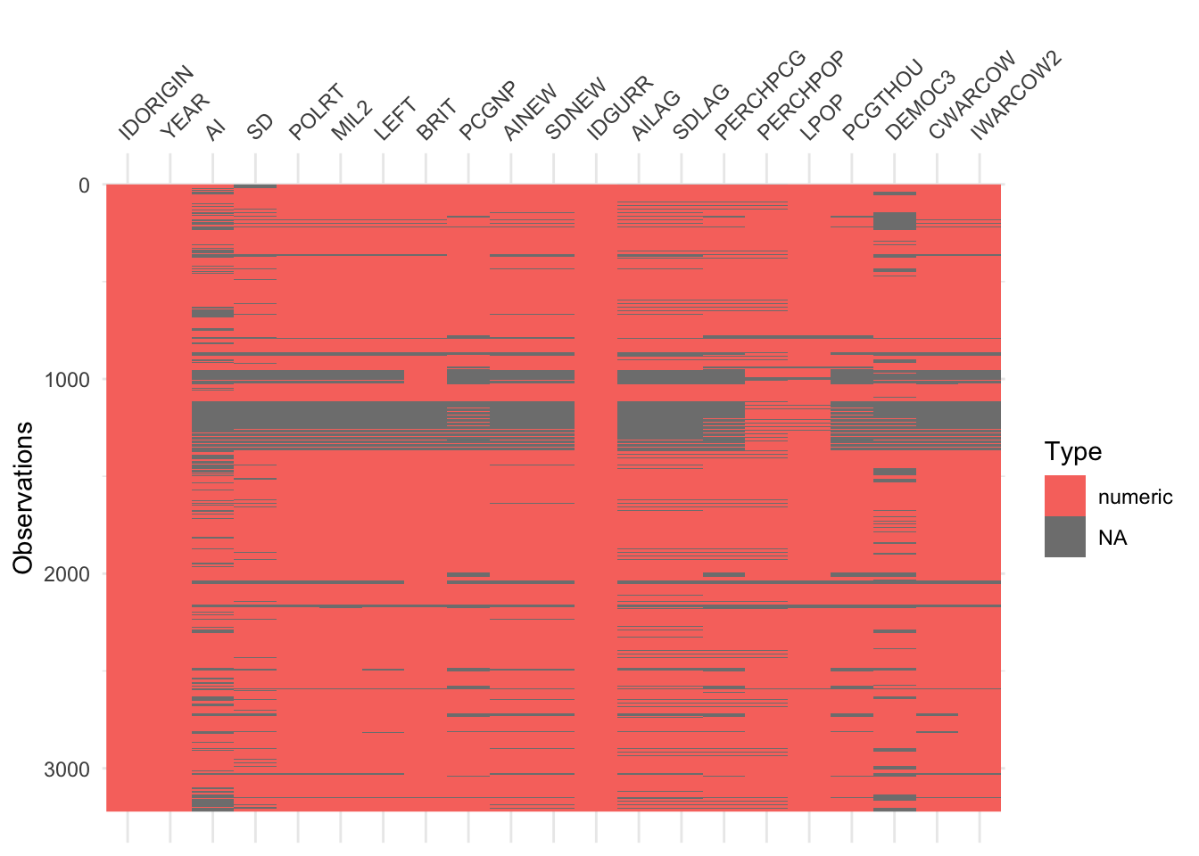
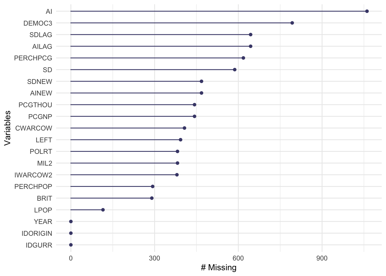
mi misstable summarize
* There are some logical restrictions that we are going to want.
* For example, we have some changes that need to be consistent
* with levels. We can deal with that; just calculate the changes
* after imputation.
mi register imputed DEMOC3
mi impute regress DEMOC3 PERCHPCG PERCHPOP LPOP CWARCOW IWARCOW2, add(10) dots force
* mi impute regress PCGTHOU DEMOC3 PERCHPOP LPOP CWARCOW IWARCOW2, add(20)
mi estimate: xtreg AINEW AILAG DEMOC3, fe
The Data: Poe, Tate, Keith 1999
Two objectives. Load the data and transform it into a pdata.frame for now.
Will allow R to answer many questions that stata’s xt commands make available. First, some basic summaries to get to balance.
summary(ISQ99_Essex)
    IDORIGIN          YEAR            AI              SD            POLRT
 Min.   :  2.0   Min.   :1976   Min.   :1.000   Min.   :1.000   Min.   :1.000
 1st Qu.:290.0   1st Qu.:1980   1st Qu.:2.000   1st Qu.:1.000   1st Qu.:2.000
 Median :435.0   Median :1984   Median :3.000   Median :2.000   Median :3.000
 Mean   :446.7   Mean   :1984   Mean   :2.753   Mean   :2.241   Mean   :3.809
 3rd Qu.:640.0   3rd Qu.:1989   3rd Qu.:3.000   3rd Qu.:3.000   3rd Qu.:6.000
 Max.   :990.0   Max.   :1993   Max.   :5.000   Max.   :5.000   Max.   :7.000
                                NA's   :1061    NA's   :587     NA's   :382
      MIL2             LEFT             BRIT            PCGNP
 Min.   :0.0000   Min.   :0.0000   Min.   :0.0000   Min.   :   52
 1st Qu.:0.0000   1st Qu.:0.0000   1st Qu.:0.0000   1st Qu.:  390
 Median :0.0000   Median :0.0000   Median :0.0000   Median : 1112
 Mean   :0.2725   Mean   :0.1764   Mean   :0.3554   Mean   : 3592
 3rd Qu.:1.0000   3rd Qu.:0.0000   3rd Qu.:1.0000   3rd Qu.: 3510
 Max.   :1.0000   Max.   :1.0000   Max.   :1.0000   Max.   :36670
 NA's   :382      NA's   :393      NA's   :290      NA's   :443
     AINEW           SDNEW           IDGURR          AILAG          SDLAG
 Min.   :1.000   Min.   :1.000   Min.   :  2.0   Min.   :1.00   Min.   :1.000
 1st Qu.:1.000   1st Qu.:1.000   1st Qu.:290.0   1st Qu.:1.00   1st Qu.:1.000
 Median :2.000   Median :2.000   Median :450.0   Median :2.00   Median :2.000
 Mean   :2.443   Mean   :2.262   Mean   :455.8   Mean   :2.45   Mean   :2.247
 3rd Qu.:3.000   3rd Qu.:3.000   3rd Qu.:663.0   3rd Qu.:3.00   3rd Qu.:3.000
 Max.   :5.000   Max.   :5.000   Max.   :990.0   Max.   :5.00   Max.   :5.000
 NA's   :468     NA's   :468                     NA's   :644    NA's   :644
    PERCHPCG          PERCHPOP            LPOP          PCGTHOU
 Min.   :-95.500   Min.   :-48.450   Min.   :11.00   Min.   : 0.050
 1st Qu.: -2.545   1st Qu.:  0.910   1st Qu.:14.51   1st Qu.: 0.390
 Median :  4.615   Median :  2.220   Median :15.59   Median : 1.110
 Mean   :  4.614   Mean   :  2.193   Mean   :15.48   Mean   : 3.592
 3rd Qu.: 11.760   3rd Qu.:  2.940   3rd Qu.:16.64   3rd Qu.: 3.510
 Max.   :128.570   Max.   :126.010   Max.   :20.89   Max.   :36.670
 NA's   :618       NA's   :293       NA's   :115     NA's   :443
     DEMOC3          CWARCOW         IWARCOW2
 Min.   : 0.000   Min.   :0.000   Min.   :0.0000
 1st Qu.: 0.000   1st Qu.:0.000   1st Qu.:0.0000
 Median : 0.000   Median :0.000   Median :0.0000
 Mean   : 3.682   Mean   :0.092   Mean   :0.0862
 3rd Qu.: 9.000   3rd Qu.:0.000   3rd Qu.:0.0000
 Max.   :10.000   Max.   :1.000   Max.   :1.0000
 NA's   :793      NA's   :407     NA's   :380
no time variation:       IDORIGIN BRIT IDGURR AILAG SDLAG PERCHPCG PERCHPOP
no individual variation: YEAR AI SD POLRT MIL2 LEFT BRIT PCGNP AINEW SDNEW AILAG SDLAG PERCHPCG PERCHPOP LPOP PCGTHOU DEMOC3 CWARCOW IWARCOW2
all NA in time dimension for at least one individual:  AI SD POLRT MIL2 LEFT BRIT PCGNP AINEW SDNEW AILAG SDLAG PERCHPCG PERCHPOP LPOP PCGTHOU DEMOC3 CWARCOW IWARCOW2
all NA in ind. dimension for at least one time period: AI SD POLRT MIL2 LEFT BRIT PCGNP AINEW SDNEW AILAG SDLAG PERCHPCG PERCHPOP LPOP PCGTHOU DEMOC3 CWARCOW IWARCOW2
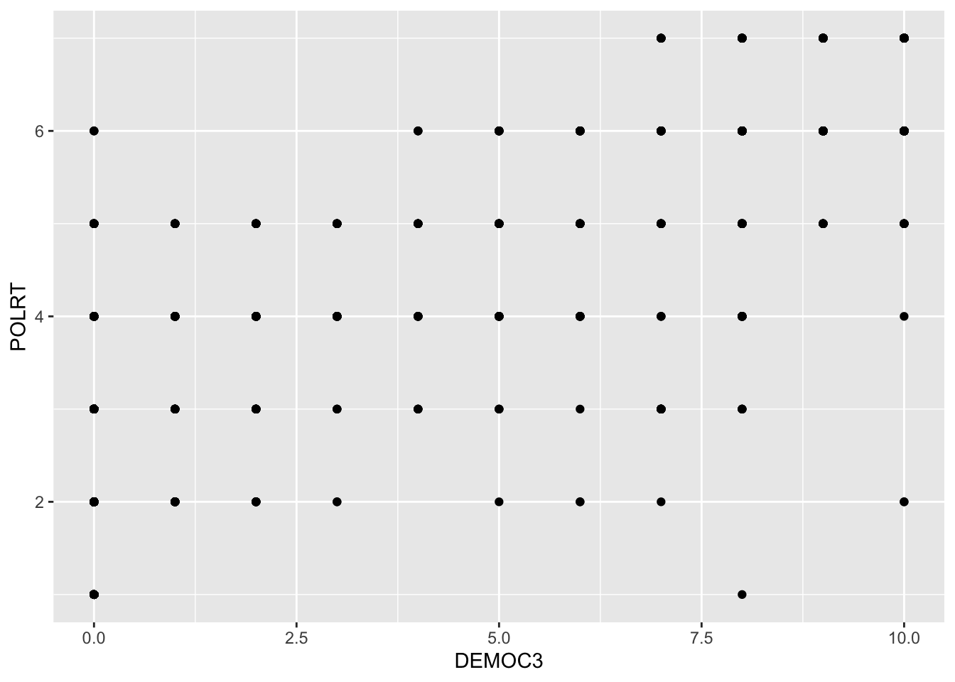
mplot <-ggplot(ISQ99_Essex, aes(x = DEMOC3, y = POLRT)) +geom_point()mplot
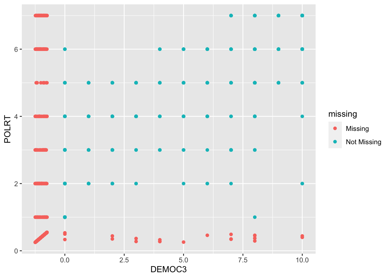
library(naniar)mplot <-ggplot(ISQ99_Essex, aes(x = DEMOC3, y = POLRT)) +geom_miss_point()mplot
Multiple Imputation: Amelia II
A simple multivariate normal is easy as long as the data are well behaved. NB: This uses none of the time series or cross-sectional dimensionality for identification.
Warning: There are observations in the data that are completely missing.
         These observations will remain unimputed in the final datasets.
-- Imputation 1 --

  1  2  3  4  5  6  7

-- Imputation 2 --

  1  2  3  4  5  6  7  8  9

-- Imputation 3 --

  1  2  3  4  5  6  7  8

-- Imputation 4 --

  1  2  3  4  5  6  7  8  9 10

-- Imputation 5 --

  1  2  3  4  5  6
Without simplifying, it crashes because there are id variables of different sorts and other things hiding in there, perfect multicollinearities exist. Even with them, we need a bit more work.
Transforms are Key
Using the cs and ts information with polytime/splinetime and intercs
Amelia output with 5 imputed datasets.
Return code: 1
Message: Normal EM convergence.
Chain Lengths:
--------------
Imputation 1: 20
Imputation 2: 20
Imputation 3: 20
Imputation 4: 20
Imputation 5: 20
Rows after Listwise Deletion: 2144
Rows after Imputation: 3222
Patterns of missingness in the data: 65
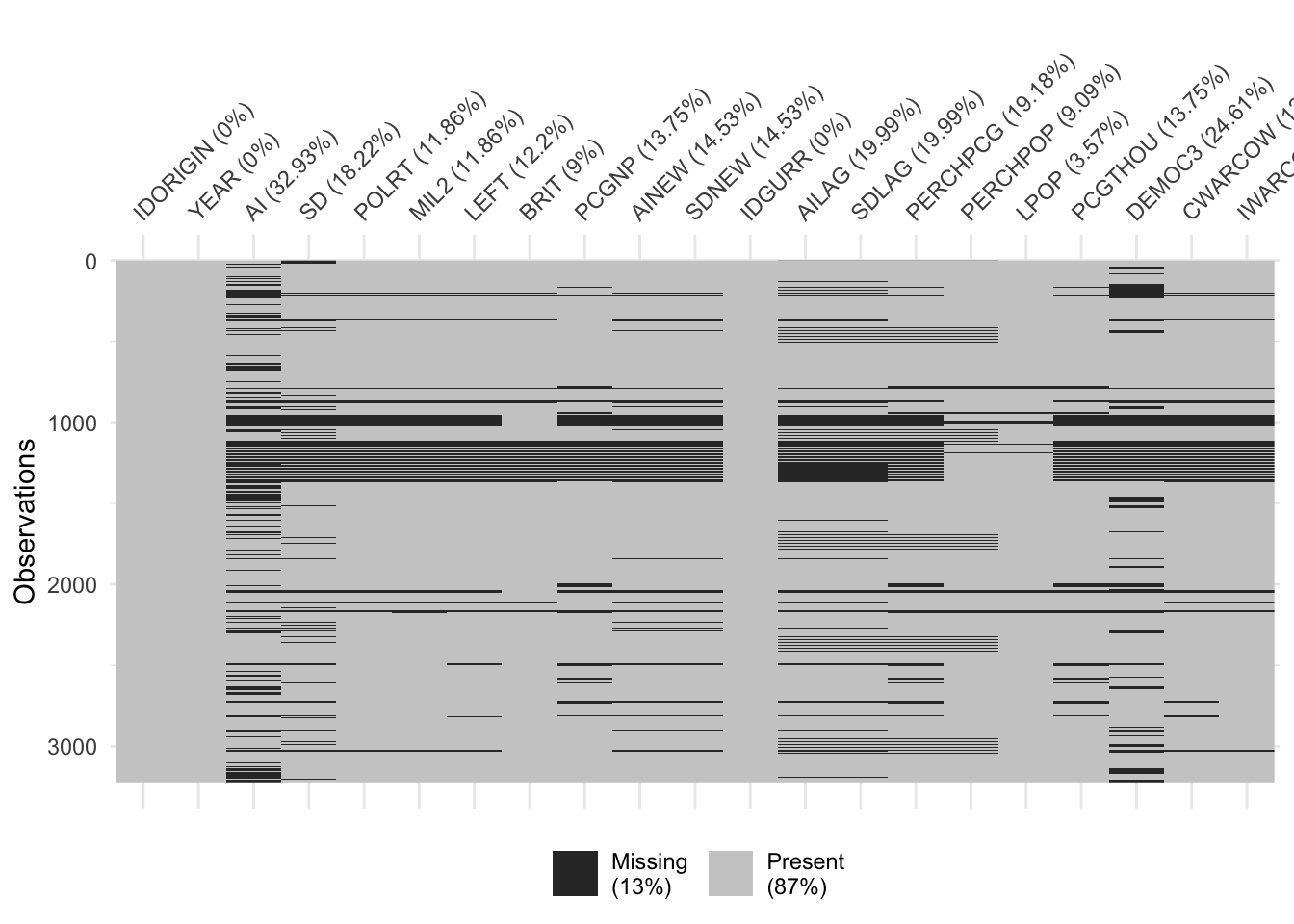
Fraction Missing for original variables:
-----------------------------------------
Fraction Missing
IDORIGIN 0.00000000
YEAR 0.00000000
POLRT 0.11855990
MIL2 0.11855990
LEFT 0.12197393
BRIT 0.09000621
PCGNP 0.13749224
AINEW 0.14525140
SDNEW 0.14525140
AILAG 0.19987585
SDLAG 0.19987585
PERCHPCG 0.19180633
PERCHPOP 0.09093731
LPOP 0.03569212
PCGTHOU 0.13749224
DEMOC3 0.24612042
CWARCOW 0.12631906
IWARCOW2 0.11793917
Now let’s analyze it.
Some Analysis
Not a correct model but a first start.
devtools::install_github("IQSS/ZeligChoice")library(ZeligChoice)Model.a2 <-zelig(AINEW ~ AILAG + MIL2 + LEFT + BRIT + CWARCOW + IWARCOW2 + PCGTHOU + PERCHPOP + DEMOC3, model ="ls", data = a.out2)
How to cite this model in Zelig:
  R Core Team. 2007.
  ls: Least Squares Regression for Continuous Dependent Variables
  in Christine Choirat, Christopher Gandrud, James Honaker, Kosuke Imai, Gary King, and Olivia Lau,
  "Zelig: Everyone's Statistical Software," https://zeligproject.org/
summary(Model.a2)
Model: Combined Imputations

             Estimate Std.Error z value Pr(>|z|)
(Intercept)  1.040136  0.055780   18.65  < 2e-16
AILAG        0.621404  0.017965   34.59  < 2e-16
MIL2         0.110257  0.035754    3.08  0.00204
LEFT        -0.074708  0.046963   -1.59  0.11166
BRIT        -0.112423  0.030393   -3.70  0.00022
CWARCOW      0.532683  0.055780    9.55  < 2e-16
IWARCOW2     0.180371  0.071370    2.53  0.01150
PCGTHOU     -0.016131  0.003344   -4.82  1.4e-06
PERCHPOP    -0.000936  0.003508   -0.27  0.78956
DEMOC3      -0.030649  0.004348   -7.05  1.8e-12

For results from individual imputed datasets, use summary(x, subset = i:j)
Statistical Warning: The GIM test suggests this model is misspecified
 (based on comparisons between classical and robust SE's; see http://j.mp/GIMtest).
 We suggest you run diagnostics to ascertain the cause, respecify the model
 and run it again.

Next step: Use 'setx' method