Slides
Two core issues remain: the spatial and the temporal. There are fewer well worked diagnostics for this than for the pure linear case owing to partial observability and/or coarse measurement in some fashion or other.
R
All of the computing will take place in the confines of pglm, a package in the spirit of plm for linear models. The help file provides an example of the familiar models. They are specified to match up with the syntax of R’s glm functions with family and link arguments.
# install.packages("pglm")
library(pglm)
## an ordered probit example
data('Fairness', package = 'pglm')
Parking <- subset(Fairness, good == 'parking')
op <- pglm(as.numeric(answer) ~ education + rule,
Parking[1:105, ],
family = ordinal('probit'), R = 5, print.level = 3,
method = 'bfgs', index = 'id', model = "random")
## a binomial (probit) example
data('UnionWage', package = 'pglm')
anb <- pglm(union ~ wage + exper + rural, UnionWage, family = binomial('probit'),
model = "pooling", method = "bfgs", print.level = 3, R = 5)
## a gaussian example on unbalanced panel data
data(Hedonic, package = "plm")
ra <- pglm(mv ~ crim + zn + indus + nox + age + rm, Hedonic, family = gaussian,
model = "random", print.level = 3, method = "nr", index = "townid")
## some count data models
data("PatentsRDUS", package="pglm")
la <- pglm(patents ~ lag(log(rd), 0:5) + scisect + log(capital72) + factor(year), PatentsRDUS,
family = negbin, model = "within", print.level = 3, method = "nr",
index = c('cusip', 'year'))
la <- pglm(patents ~ lag(log(rd), 0:5) + scisect + log(capital72) + factor(year), PatentsRDUS,
family = poisson, model = "pooling", index = c("cusip", "year"),
print.level = 0, method="nr")
## a tobit example
data("HealthIns", package="pglm")
HealthIns$med2 <- HealthIns$med / 1000
HealthIns2 <- HealthIns[-2209, ]
set.seed(2)
subs <- sample(1:20186, 200, replace = FALSE)
HealthIns2 <- HealthIns2[subs, ]
la <- pglm(med ~ mdu + disease + age, HealthIns2,
model = 'random', family = 'tobit', print.level = 0,
method = 'nr', R = 5)
Stata
Stata separates out the commands by family/link combination. So there are xtprobit and xtlogit for binary. xtoprobit for ordered probit models and xtologit [with random effects] for ordered outcomes.
Events
A Stata do file on the box is replicated here. First, a use of regular old glm.
library (haven)<- read_dta (url ("https://github.com/robertwwalker/Essex-Data/raw/main/Patents.dta" )).1 <- glm (PAT~ LOGR+ LOGR1+ LOGR2+ LOGR3+ LOGR4+ LOGR5+ dyear2+ dyear3+ dyear4+ dyear5, data= Patents, family= "poisson" )summary (Mod.1 )
Call:
glm(formula = PAT ~ LOGR + LOGR1 + LOGR2 + LOGR3 + LOGR4 + LOGR5 +
    dyear2 + dyear3 + dyear4 + dyear5, family = "poisson", data = Patents)

Deviance Residuals:
     Min        1Q    Median        3Q       Max
-24.1602   -3.0131   -1.6689    0.2972   23.3629

Coefficients:
            Estimate Std. Error z value Pr(>|z|)
(Intercept)  1.82831    0.01253 145.861  < 2e-16 ***
LOGR         0.15251    0.02939   5.189 2.11e-07 ***
LOGR1        0.02198    0.04083   0.538 0.590297
LOGR2        0.04369    0.03802   1.149 0.250557
LOGR3        0.08272    0.03568   2.318 0.020427 *
LOGR4        0.10397    0.03176   3.274 0.001061 **
LOGR5        0.30109    0.02063  14.594  < 2e-16 ***
dyear2      -0.04399    0.01320  -3.332 0.000862 ***
dyear3      -0.06043    0.01343  -4.499 6.81e-06 ***
dyear4      -0.18925    0.01368 -13.830  < 2e-16 ***
dyear5      -0.22979    0.01363 -16.854  < 2e-16 ***
---
Signif. codes:  0 '***' 0.001 '**' 0.01 '*' 0.05 '.' 0.1 ' ' 1

(Dispersion parameter for poisson family taken to be 1)

    Null deviance: 144500  on 1729  degrees of freedom
Residual deviance:  33745  on 1719  degrees of freedom
AIC: 39807

Number of Fisher Scoring iterations: 5
library (MASS).2 <- glm.nb (PAT~ LOGR+ LOGR1+ LOGR2+ LOGR3+ LOGR4+ LOGR5+ dyear2+ dyear3+ dyear4+ dyear5, data= Patents)summary (Mod.2 )
Call:
glm.nb(formula = PAT ~ LOGR + LOGR1 + LOGR2 + LOGR3 + LOGR4 +
    LOGR5 + dyear2 + dyear3 + dyear4 + dyear5, data = Patents,
    init.theta = 1.276776486, link = log)

Deviance Residuals:
    Min       1Q   Median       3Q      Max
-2.6541  -1.0412  -0.3894   0.2827   4.3518

Coefficients:
            Estimate Std. Error z value Pr(>|z|)
(Intercept)  1.19343    0.05851  20.396  < 2e-16 ***
LOGR         0.40148    0.11591   3.464 0.000533 ***
LOGR1       -0.11198    0.15672  -0.714 0.474920
LOGR2        0.11039    0.14742   0.749 0.453957
LOGR3        0.08770    0.13696   0.640 0.521938
LOGR4        0.24389    0.12259   1.989 0.046657 *
LOGR5        0.17263    0.08478   2.036 0.041729 *
dyear2      -0.05346    0.07726  -0.692 0.488943
dyear3      -0.05482    0.07790  -0.704 0.481611
dyear4      -0.11764    0.07768  -1.514 0.129941
dyear5      -0.22006    0.07764  -2.835 0.004589 **
---
Signif. codes:  0 '***' 0.001 '**' 0.01 '*' 0.05 '.' 0.1 ' ' 1

(Dispersion parameter for Negative Binomial(1.2768) family taken to be 1)

    Null deviance: 7202.0  on 1729  degrees of freedom
Residual deviance: 1967.8  on 1719  degrees of freedom
AIC: 11594

Number of Fisher Scoring iterations: 1

              Theta:  1.2768
          Std. Err.:  0.0558

 2 x log-likelihood:  -11570.1870
Loading required package: maxLik
Loading required package: miscTools
Please cite the 'maxLik' package as:
Henningsen, Arne and Toomet, Ott (2011). maxLik: A package for maximum likelihood estimation in R. Computational Statistics 26(3), 443-458. DOI 10.1007/s00180-010-0217-1.

If you have questions, suggestions, or comments regarding the 'maxLik' package, please use a forum or 'tracker' at maxLik's R-Forge site:
https://r-forge.r-project.org/projects/maxlik/
Loading required package: plm
<- pdata.frame (Patents, index= c ("id" ,"YEAR" )).3 A <- pglm (PAT~ LOGR+ LOGR1+ LOGR2+ LOGR3+ LOGR4+ LOGR5+ dyear2+ dyear3+ dyear4+ dyear5+ LOGK+ SCISECT, Patents.pdata, effect= "individual" , model= "random" , family= "poisson" )summary (Mod.3 A)
--------------------------------------------
Maximum Likelihood estimation
Newton-Raphson maximisation, 4 iterations
Return code 8: successive function values within relative tolerance limit (reltol)
Log-Likelihood: -5234.927
14  free parameters
Estimates:
            Estimate Std. error t value  Pr(> t)
(Intercept)  0.41079    0.14674   2.799 0.005121 **
LOGR         0.40345    0.04350   9.274  < 2e-16 ***
LOGR1       -0.04618    0.04822  -0.958 0.338277
LOGR2        0.10792    0.04471   2.414 0.015788 *
LOGR3        0.02977    0.04132   0.720 0.471221
LOGR4        0.01070    0.03771   0.284 0.776679
LOGR5        0.04061    0.03157   1.286 0.198364
dyear2      -0.04496    0.01313  -3.425 0.000616 ***
dyear3      -0.04839    0.01340  -3.610 0.000306 ***
dyear4      -0.17416    0.01397 -12.467  < 2e-16 ***
dyear5      -0.22590    0.01466 -15.404  < 2e-16 ***
LOGK         0.29169    0.03934   7.415 1.21e-13 ***
SCISECT      0.25700    0.11227   2.289 0.022074 *
sigma        1.16969    0.09471  12.350  < 2e-16 ***
---
Signif. codes:  0 '***' 0.001 '**' 0.01 '*' 0.05 '.' 0.1 ' ' 1
--------------------------------------------
.3 B <- pglm (PAT~ LOGR+ LOGR1+ LOGR2+ LOGR3+ LOGR4+ LOGR5+ dyear2+ dyear3+ dyear4+ dyear5, Patents.pdata, effect= "individual" , model= "random" , family= "poisson" )summary (Mod.3 B)
--------------------------------------------
Maximum Likelihood estimation
Newton-Raphson maximisation, 5 iterations
Return code 1: gradient close to zero (gradtol)
Log-Likelihood: -5263.611
12  free parameters
Estimates:
             Estimate Std. error t value  Pr(> t)
(Intercept)  1.402861   0.067052  20.922  < 2e-16 ***
LOGR         0.476575   0.042263  11.276  < 2e-16 ***
LOGR1       -0.007708   0.047934  -0.161 0.872242
LOGR2        0.136413   0.044734   3.049 0.002293 **
LOGR3        0.059191   0.041279   1.434 0.151598
LOGR4        0.027518   0.037601   0.732 0.464267
LOGR5        0.082547   0.030977   2.665 0.007704 **
dyear2      -0.046879   0.013131  -3.570 0.000357 ***
dyear3      -0.056088   0.013362  -4.198  2.7e-05 ***
dyear4      -0.190312   0.013789 -13.802  < 2e-16 ***
dyear5      -0.252677   0.014197 -17.798  < 2e-16 ***
sigma        1.154854   0.094192  12.261  < 2e-16 ***
---
Signif. codes:  0 '***' 0.001 '**' 0.01 '*' 0.05 '.' 0.1 ' ' 1
--------------------------------------------
.3 C <- pglm (PAT~ LOGR+ LOGR1+ LOGR2+ LOGR3+ LOGR4+ LOGR5+ dyear2+ dyear3+ dyear4+ dyear5+ LOGK+ SCISECT-1 , Patents.pdata, effect= "individual" , model= "random" , family= "poisson" )summary (Mod.3 C)
--------------------------------------------
Maximum Likelihood estimation
Newton-Raphson maximisation, 4 iterations
Return code 1: gradient close to zero (gradtol)
Log-Likelihood: -5238.845
13  free parameters
Estimates:
         Estimate Std. error t value  Pr(> t)
LOGR     0.382042   0.042877   8.910  < 2e-16 ***
LOGR1   -0.055620   0.048157  -1.155 0.248098
LOGR2    0.100308   0.044621   2.248 0.024576 *
LOGR3    0.020949   0.041203   0.508 0.611146
LOGR4    0.005334   0.037709   0.141 0.887523
LOGR5    0.028364   0.031336   0.905 0.365383
dyear2  -0.042732   0.013109  -3.260 0.001115 **
dyear3  -0.044442   0.013332  -3.333 0.000858 ***
dyear4  -0.167871   0.013796 -12.168  < 2e-16 ***
dyear5  -0.216749   0.014303 -15.154  < 2e-16 ***
LOGK     0.388567   0.019946  19.481  < 2e-16 ***
SCISECT  0.419111   0.097521   4.298 1.73e-05 ***
sigma    1.117773   0.088520  12.627  < 2e-16 ***
---
Signif. codes:  0 '***' 0.001 '**' 0.01 '*' 0.05 '.' 0.1 ' ' 1
--------------------------------------------
.4 A <- pglm (PAT~ LOGR+ LOGR1+ LOGR2+ LOGR3+ LOGR4+ LOGR5+ dyear2+ dyear3+ dyear4+ dyear5+ LOGK+ SCISECT, Patents.pdata, effect= "individual" , model= "random" , family= "negbin" )summary (Mod.4 A)
--------------------------------------------
Maximum Likelihood estimation
Newton-Raphson maximisation, 6 iterations
Return code 1: gradient close to zero (gradtol)
Log-Likelihood: -4948.494
15  free parameters
Estimates:
             Estimate Std. error t value  Pr(> t)
(Intercept)  0.899562   0.168111   5.351 8.75e-08 ***
LOGR         0.350312   0.065282   5.366 8.04e-08 ***
LOGR1       -0.003032   0.075092  -0.040 0.967796
LOGR2        0.104988   0.068849   1.525 0.127284
LOGR3        0.016352   0.063638   0.257 0.797210
LOGR4        0.035942   0.058716   0.612 0.540445
LOGR5        0.071832   0.048289   1.488 0.136867
dyear2      -0.043674   0.021343  -2.046 0.040734 *
dyear3      -0.055660   0.021857  -2.547 0.010881 *
dyear4      -0.183105   0.022718  -8.060 7.64e-16 ***
dyear5      -0.230044   0.023152  -9.936  < 2e-16 ***
LOGK         0.161937   0.041787   3.875 0.000107 ***
SCISECT      0.117642   0.106616   1.103 0.269848
a            2.685210   0.258163  10.401  < 2e-16 ***
b            2.015688   0.217631   9.262  < 2e-16 ***
---
Signif. codes:  0 '***' 0.001 '**' 0.01 '*' 0.05 '.' 0.1 ' ' 1
--------------------------------------------
.4 B <- pglm (PAT~ LOGR+ LOGR1+ LOGR2+ LOGR3+ LOGR4+ LOGR5+ dyear2+ dyear3+ dyear4+ dyear5, Patents.pdata, effect= "individual" , model= "random" , family= "negbin" )summary (Mod.4 B)
--------------------------------------------
Maximum Likelihood estimation
Newton-Raphson maximisation, 6 iterations
Return code 1: gradient close to zero (gradtol)
Log-Likelihood: -4956.259
13  free parameters
Estimates:
            Estimate Std. error t value  Pr(> t)
(Intercept)  1.39944    0.10060  13.910  < 2e-16 ***
LOGR         0.38762    0.06492   5.970 2.37e-09 ***
LOGR1        0.01833    0.07597   0.241  0.80935
LOGR2        0.12909    0.06972   1.852  0.06408 .
LOGR3        0.02469    0.06446   0.383  0.70172
LOGR4        0.05775    0.05873   0.983  0.32544
LOGR5        0.10003    0.04750   2.106  0.03521 *
dyear2      -0.04671    0.02180  -2.142  0.03219 *
dyear3      -0.06512    0.02223  -2.930  0.00339 **
dyear4      -0.20006    0.02282  -8.765  < 2e-16 ***
dyear5      -0.25096    0.02298 -10.921  < 2e-16 ***
a            2.64396    0.25190  10.496  < 2e-16 ***
b            2.02183    0.21889   9.237  < 2e-16 ***
---
Signif. codes:  0 '***' 0.001 '**' 0.01 '*' 0.05 '.' 0.1 ' ' 1
--------------------------------------------
.4 C <- pglm (PAT~ LOGR+ LOGR1+ LOGR2+ LOGR3+ LOGR4+ LOGR5+ dyear2+ dyear3+ dyear4+ dyear5+ LOGK+ SCISECT-1 , Patents.pdata, effect= "individual" , model= "random" , family= "negbin" )summary (Mod.4 C)
--------------------------------------------
Maximum Likelihood estimation
Newton-Raphson maximisation, 6 iterations
Return code 1: gradient close to zero (gradtol)
Log-Likelihood: -4963.305
14  free parameters
Estimates:
         Estimate Std. error t value  Pr(> t)
LOGR     0.296803   0.066943   4.434 9.26e-06 ***
LOGR1   -0.005170   0.078300  -0.066   0.9474
LOGR2    0.085684   0.071482   1.199   0.2307
LOGR3    0.004177   0.065959   0.063   0.9495
LOGR4    0.010518   0.060898   0.173   0.8629
LOGR5    0.048459   0.050342   0.963   0.3357
dyear2  -0.032498   0.021569  -1.507   0.1319
dyear3  -0.037854   0.021894  -1.729   0.0838 .
dyear4  -0.159944   0.022586  -7.082 1.42e-12 ***
dyear5  -0.201171   0.022791  -8.827  < 2e-16 ***
LOGK     0.343399   0.027143  12.652  < 2e-16 ***
SCISECT  0.427951   0.089606   4.776 1.79e-06 ***
a        2.435387   0.225784  10.786  < 2e-16 ***
b        2.154018   0.240574   8.954  < 2e-16 ***
---
Signif. codes:  0 '***' 0.001 '**' 0.01 '*' 0.05 '.' 0.1 ' ' 1
--------------------------------------------
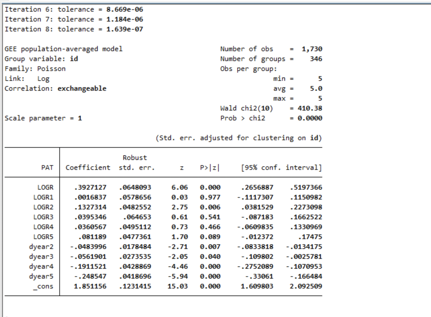
The GEE
library (geepack)<- geeglm (PAT~ LOGR+ LOGR1+ LOGR2+ LOGR3+ LOGR4+ LOGR5+ dyear2+ dyear3+ dyear4+ dyear5, data= Patents, id= id, corstr= "exchangeable" , family= poisson)summary (gee.Mod)
Call:
geeglm(formula = PAT ~ LOGR + LOGR1 + LOGR2 + LOGR3 + LOGR4 +
    LOGR5 + dyear2 + dyear3 + dyear4 + dyear5, family = poisson,
    data = Patents, id = id, corstr = "exchangeable")

 Coefficients:
             Estimate   Std.err    Wald Pr(>|W|)
(Intercept)  1.851156  0.122963 226.638  < 2e-16 ***
LOGR         0.392713  0.064716  36.824 1.29e-09 ***
LOGR1        0.001683  0.057782   0.001  0.97677
LOGR2        0.132732  0.048185   7.588  0.00588 **
LOGR3        0.039535  0.064560   0.375  0.54029
LOGR4        0.036056  0.049440   0.532  0.46582
LOGR5        0.081190  0.047667   2.901  0.08851 .
dyear2      -0.048400  0.017823   7.375  0.00661 **
dyear3      -0.056190  0.027314   4.232  0.03967 *
dyear4      -0.191152  0.042825  19.923 8.06e-06 ***
dyear5      -0.248547  0.041809  35.341 2.77e-09 ***
---
Signif. codes:  0 '***' 0.001 '**' 0.01 '*' 0.05 '.' 0.1 ' ' 1

Correlation structure = exchangeable
Estimated Scale Parameters:

            Estimate Std.err
(Intercept)    22.57   4.102
  Link = identity

Estimated Correlation Parameters:
      Estimate Std.err
alpha   0.8983 0.06245
Number of clusters:   346  Maximum cluster size: 5
<- geeglm (PAT~ LOGR+ LOGR1+ LOGR2+ LOGR3+ LOGR4+ LOGR5+ dyear2+ dyear3+ dyear4+ dyear5, data= Patents, id= id, corstr= "ar1" , family= poisson)summary (gee.Mod)
Call:
geeglm(formula = PAT ~ LOGR + LOGR1 + LOGR2 + LOGR3 + LOGR4 +
    LOGR5 + dyear2 + dyear3 + dyear4 + dyear5, family = poisson,
    data = Patents, id = id, corstr = "ar1")

 Coefficients:
            Estimate Std.err   Wald Pr(>|W|)
(Intercept)   1.8121  0.1270 203.72  < 2e-16 ***
LOGR          0.3096  0.0554  31.17  2.4e-08 ***
LOGR1         0.0254  0.0549   0.21   0.6435
LOGR2         0.1624  0.0518   9.82   0.0017 **
LOGR3         0.0801  0.0564   2.02   0.1555
LOGR4         0.0793  0.0446   3.16   0.0756 .
LOGR5         0.0408  0.0411   0.99   0.3200
dyear2       -0.0494  0.0175   8.01   0.0047 **
dyear3       -0.0542  0.0266   4.14   0.0419 *
dyear4       -0.1817  0.0427  18.08  2.1e-05 ***
dyear5       -0.2333  0.0409  32.48  1.2e-08 ***
---
Signif. codes:  0 '***' 0.001 '**' 0.01 '*' 0.05 '.' 0.1 ' ' 1

Correlation structure = ar1
Estimated Scale Parameters:

            Estimate Std.err
(Intercept)     22.3    4.02
  Link = identity

Estimated Correlation Parameters:
      Estimate Std.err
alpha    0.948  0.0265
Number of clusters:   346  Maximum cluster size: 5
And an anova…
Analysis of 'Wald statistic' Table
Model: poisson, link: log
Response: PAT
Terms added sequentially (first to last)

       Df  X2 P(>|Chi|)
LOGR    1 368   < 2e-16 ***
LOGR1   1  23   1.9e-06 ***
LOGR2   1  19   1.4e-05 ***
LOGR3   1  16   5.8e-05 ***
LOGR4   1   7   0.00708 **
LOGR5   1   1   0.28590
dyear2  1   4   0.05740 .
dyear3  1  11   0.00099 ***
dyear4  1   0   0.67359
dyear5  1  32   1.2e-08 ***
---
Signif. codes:  0 '***' 0.001 '**' 0.01 '*' 0.05 '.' 0.1 ' ' 1
BKT and Carter-Signorino
Load the data
<- read_dta (url ("https://github.com/robertwwalker/Essex-Data/raw/main/bkt98ajps.dta" )).1 <- glm (dispute~ dem+ growth+ allies+ contig+ capratio+ trade, family= binomial ("logit" ), data= BKT.data)summary (Mod.1 )
Call:
glm(formula = dispute ~ dem + growth + allies + contig + capratio +
    trade, family = binomial("logit"), data = BKT.data)

Deviance Residuals:
   Min      1Q  Median      3Q     Max
-0.748  -0.319  -0.261  -0.152   4.096

Coefficients:
             Estimate Std. Error z value Pr(>|z|)
(Intercept) -3.29e+00   7.92e-02  -41.54  < 2e-16 ***
dem         -4.97e-02   7.38e-03   -6.73  1.7e-11 ***
growth      -2.23e-02   8.52e-03   -2.62   0.0088 **
allies      -8.21e-01   8.00e-02  -10.26  < 2e-16 ***
contig       1.31e+00   7.96e-02   16.49  < 2e-16 ***
capratio    -3.07e-03   4.17e-04   -7.37  1.8e-13 ***
trade       -6.61e+01   1.34e+01   -4.92  8.6e-07 ***
---
Signif. codes:  0 '***' 0.001 '**' 0.01 '*' 0.05 '.' 0.1 ' ' 1

(Dispersion parameter for binomial family taken to be 1)

    Null deviance: 7719.2  on 20989  degrees of freedom
Residual deviance: 6955.1  on 20983  degrees of freedom
AIC: 6969

Number of Fisher Scoring iterations: 8
.1 B <- glm (dispute~ dem+ growth+ allies+ contig+ capratio+ trade+ as.factor (py), family= binomial ("logit" ), data= BKT.data)
Warning: glm.fit: fitted probabilities numerically 0 or 1 occurred
Call:
glm(formula = dispute ~ dem + growth + allies + contig + capratio +
    trade + as.factor(py), family = binomial("logit"), data = BKT.data)

Deviance Residuals:
   Min      1Q  Median      3Q     Max
-1.362  -0.225  -0.140  -0.080   3.988

Coefficients:
                 Estimate Std. Error z value Pr(>|z|)
(Intercept)     -9.43e-01   9.28e-02  -10.16  < 2e-16 ***
dem             -5.47e-02   8.00e-03   -6.84  8.0e-12 ***
growth          -1.15e-02   9.24e-03   -1.24  0.21492
allies          -4.71e-01   9.00e-02   -5.23  1.7e-07 ***
contig           6.99e-01   8.93e-02    7.82  5.3e-15 ***
capratio        -3.03e-03   4.17e-04   -7.28  3.3e-13 ***
trade           -1.27e+01   1.05e+01   -1.21  0.22735
as.factor(py)2  -2.04e+00   1.41e-01  -14.48  < 2e-16 ***
as.factor(py)3  -2.15e+00   1.54e-01  -13.92  < 2e-16 ***
as.factor(py)4  -2.37e+00   1.74e-01  -13.64  < 2e-16 ***
as.factor(py)5  -2.62e+00   2.01e-01  -13.04  < 2e-16 ***
as.factor(py)6  -3.09e+00   2.52e-01  -12.25  < 2e-16 ***
as.factor(py)7  -3.08e+00   2.52e-01  -12.21  < 2e-16 ***
as.factor(py)8  -3.00e+00   2.46e-01  -12.23  < 2e-16 ***
as.factor(py)9  -2.95e+00   2.46e-01  -11.98  < 2e-16 ***
as.factor(py)10 -3.24e+00   2.86e-01  -11.32  < 2e-16 ***
as.factor(py)11 -3.45e+00   3.24e-01  -10.66  < 2e-16 ***
as.factor(py)12 -3.32e+00   3.10e-01  -10.72  < 2e-16 ***
as.factor(py)13 -3.92e+00   4.14e-01   -9.46  < 2e-16 ***
as.factor(py)14 -4.56e+00   5.82e-01   -7.84  4.6e-15 ***
as.factor(py)15 -4.58e+00   5.82e-01   -7.87  3.5e-15 ***
as.factor(py)16 -3.45e+00   3.41e-01  -10.12  < 2e-16 ***
as.factor(py)17 -4.22e+00   5.05e-01   -8.35  < 2e-16 ***
as.factor(py)18 -5.59e+00   1.00e+00   -5.57  2.5e-08 ***
as.factor(py)19 -3.61e+00   3.85e-01   -9.36  < 2e-16 ***
as.factor(py)20 -3.95e+00   4.53e-01   -8.71  < 2e-16 ***
as.factor(py)21 -4.80e+00   7.11e-01   -6.74  1.5e-11 ***
as.factor(py)22 -4.31e+00   5.82e-01   -7.39  1.4e-13 ***
as.factor(py)23 -4.13e+00   5.83e-01   -7.08  1.4e-12 ***
as.factor(py)24 -3.99e+00   5.83e-01   -6.84  7.7e-12 ***
as.factor(py)25 -1.76e+01   3.31e+02   -0.05  0.95752
as.factor(py)26 -2.97e+00   4.19e-01   -7.10  1.2e-12 ***
as.factor(py)27 -1.76e+01   3.85e+02   -0.05  0.96353
as.factor(py)28 -1.76e+01   3.83e+02   -0.05  0.96347
as.factor(py)29 -3.92e+00   7.14e-01   -5.49  3.9e-08 ***
as.factor(py)30 -3.42e+00   5.86e-01   -5.84  5.2e-09 ***
as.factor(py)31 -4.41e+00   1.01e+00   -4.39  1.1e-05 ***
as.factor(py)32 -3.57e+00   7.15e-01   -4.99  6.0e-07 ***
as.factor(py)33 -4.07e+00   1.01e+00   -4.05  5.2e-05 ***
as.factor(py)34 -3.31e+00   7.16e-01   -4.61  3.9e-06 ***
as.factor(py)35 -3.83e+00   1.01e+00   -3.81  0.00014 ***
---
Signif. codes:  0 '***' 0.001 '**' 0.01 '*' 0.05 '.' 0.1 ' ' 1

(Dispersion parameter for binomial family taken to be 1)

    Null deviance: 7719.2  on 20989  degrees of freedom
Residual deviance: 5109.4  on 20949  degrees of freedom
AIC: 5191

Number of Fisher Scoring iterations: 17
.1 C <- glm (dispute~ dem+ growth+ allies+ contig+ capratio+ trade+ py+ pys1+ pys2+ pys3, family= binomial ("logit" ), data= BKT.data)summary (Mod.1 C)
Call:
glm(formula = dispute ~ dem + growth + allies + contig + capratio +
    trade + py + pys1 + pys2 + pys3, family = binomial("logit"),
    data = BKT.data)

Deviance Residuals:
   Min      1Q  Median      3Q     Max
-1.349  -0.221  -0.138  -0.092   4.063

Coefficients:
             Estimate Std. Error z value Pr(>|z|)
(Intercept)  8.50e-01   1.60e-01    5.31  1.1e-07 ***
dem         -5.46e-02   7.97e-03   -6.84  7.7e-12 ***
growth      -1.15e-02   9.20e-03   -1.25     0.21
allies      -4.70e-01   8.96e-02   -5.25  1.5e-07 ***
contig       6.94e-01   8.90e-02    7.79  6.6e-15 ***
capratio    -3.04e-03   4.17e-04   -7.29  3.0e-13 ***
trade       -1.29e+01   1.05e+01   -1.23     0.22
py          -1.82e+00   1.11e-01  -16.30  < 2e-16 ***
pys1        -2.45e-01   2.61e-02   -9.37  < 2e-16 ***
pys2         7.92e-02   1.09e-02    7.24  4.5e-13 ***
pys3        -1.09e-02   2.76e-03   -3.96  7.5e-05 ***
---
Signif. codes:  0 '***' 0.001 '**' 0.01 '*' 0.05 '.' 0.1 ' ' 1

(Dispersion parameter for binomial family taken to be 1)

    Null deviance: 7719.2  on 20989  degrees of freedom
Residual deviance: 5165.8  on 20979  degrees of freedom
AIC: 5188

Number of Fisher Scoring iterations: 8
.2 A <- glm (dispute~ dem+ growth+ allies+ contig+ capratio+ trade, family= binomial ("logit" ), subset = contdisp!= 1 , data= BKT.data)summary (Mod.2 A)
Call:
glm(formula = dispute ~ dem + growth + allies + contig + capratio +
    trade, family = binomial("logit"), data = BKT.data, subset = contdisp !=
    1)

Deviance Residuals:
   Min      1Q  Median      3Q     Max
-0.520  -0.218  -0.169  -0.120   3.868

Coefficients:
             Estimate Std. Error z value Pr(>|z|)
(Intercept) -4.33e+00   1.15e-01  -37.78  < 2e-16 ***
dem         -4.01e-02   1.01e-02   -3.99  6.7e-05 ***
growth      -3.43e-02   1.25e-02   -2.74   0.0062 **
allies      -4.80e-01   1.13e-01   -4.25  2.1e-05 ***
contig       1.35e+00   1.21e-01   11.20  < 2e-16 ***
capratio    -1.96e-03   5.01e-04   -3.92  9.0e-05 ***
trade       -2.11e+01   1.13e+01   -1.86   0.0623 .
---
Signif. codes:  0 '***' 0.001 '**' 0.01 '*' 0.05 '.' 0.1 ' ' 1

(Dispersion parameter for binomial family taken to be 1)

    Null deviance: 3978.5  on 20447  degrees of freedom
Residual deviance: 3693.8  on 20441  degrees of freedom
AIC: 3708

Number of Fisher Scoring iterations: 9
.2 B <- glm (dispute~ dem+ growth+ allies+ contig+ capratio+ trade+ py+ pys1+ pys2+ pys3, family= binomial ("logit" ), subset = contdisp!= 1 , data= BKT.data)summary (Mod.2 B)
Call:
glm(formula = dispute ~ dem + growth + allies + contig + capratio +
    trade + py + pys1 + pys2 + pys3, family = binomial("logit"),
    data = BKT.data, subset = contdisp != 1)

Deviance Residuals:
   Min      1Q  Median      3Q     Max
-0.734  -0.210  -0.135  -0.098   3.732

Coefficients:
             Estimate Std. Error z value Pr(>|z|)
(Intercept) -3.956674   0.297828  -13.29  < 2e-16 ***
dem         -0.038809   0.010046   -3.86  0.00011 ***
growth      -0.040144   0.012502   -3.21  0.00132 **
allies      -0.365957   0.114272   -3.20  0.00136 **
contig       0.993251   0.124133    8.00  1.2e-15 ***
capratio    -0.002289   0.000523   -4.38  1.2e-05 ***
trade       -3.809220   9.679795   -0.39  0.69393
py           0.390965   0.157920    2.48  0.01330 *
pys1         0.089719   0.031787    2.82  0.00477 **
pys2        -0.028888   0.012634   -2.29  0.02222 *
pys3         0.003314   0.002974    1.11  0.26513
---
Signif. codes:  0 '***' 0.001 '**' 0.01 '*' 0.05 '.' 0.1 ' ' 1

(Dispersion parameter for binomial family taken to be 1)

    Null deviance: 3978.5  on 20447  degrees of freedom
Residual deviance: 3502.8  on 20437  degrees of freedom
AIC: 3525

Number of Fisher Scoring iterations: 9
.3 A <- glm (dispute~ dem+ growth+ allies+ contig+ capratio+ trade+ py+ pys1+ pys2+ pys3, family= binomial ("logit" ), subset = prefail< 1 , data= BKT.data)summary (Mod.3 A)
Call:
glm(formula = dispute ~ dem + growth + allies + contig + capratio +
    trade + py + pys1 + pys2 + pys3, family = binomial("logit"),
    data = BKT.data, subset = prefail < 1)

Deviance Residuals:
   Min      1Q  Median      3Q     Max
-0.682  -0.159  -0.109  -0.081   3.856

Coefficients:
             Estimate Std. Error z value Pr(>|z|)
(Intercept) -2.132791   0.369090   -5.78  7.5e-09 ***
dem         -0.046143   0.013330   -3.46  0.00054 ***
growth      -0.022954   0.017754   -1.29  0.19604
allies      -0.423113   0.163691   -2.58  0.00974 **
contig       1.105361   0.172537    6.41  1.5e-10 ***
capratio    -0.001916   0.000601   -3.19  0.00142 **
trade       -3.553603  11.726412   -0.30  0.76186
py          -1.081689   0.235688   -4.59  4.4e-06 ***
pys1        -0.183730   0.050096   -3.67  0.00024 ***
pys2         0.069295   0.019788    3.50  0.00046 ***
pys3        -0.013987   0.004484   -3.12  0.00181 **
---
Signif. codes:  0 '***' 0.001 '**' 0.01 '*' 0.05 '.' 0.1 ' ' 1

(Dispersion parameter for binomial family taken to be 1)

    Null deviance: 2183.3  on 16990  degrees of freedom
Residual deviance: 1928.1  on 16980  degrees of freedom
AIC: 1950

Number of Fisher Scoring iterations: 9
Carter and Signorino
Use a Taylor series to clean this up with a suggestion that no baseline hazard is more than cubic [two inflection points].
<- glm (dispute~ dem+ growth+ allies+ contig+ capratio+ trade+ prefail+ py+ I (py^ 2 )+ I (py^ 3 ), family= binomial ("logit" ), data= BKT.data)summary (Mod.CS)
Call:
glm(formula = dispute ~ dem + growth + allies + contig + capratio +
    trade + prefail + py + I(py^2) + I(py^3), family = binomial("logit"),
    data = BKT.data)

Deviance Residuals:
   Min      1Q  Median      3Q     Max
-2.576  -0.192  -0.128  -0.092   3.754

Coefficients:
             Estimate Std. Error z value Pr(>|z|)
(Intercept) -1.14e+00   1.18e-01   -9.64  < 2e-16 ***
dem         -4.09e-02   8.23e-03   -4.97  6.7e-07 ***
growth      -2.44e-02   9.55e-03   -2.56   0.0105 *
allies      -2.67e-01   9.20e-02   -2.90   0.0038 **
contig       6.62e-01   9.20e-02    7.19  6.4e-13 ***
capratio    -2.00e-03   3.71e-04   -5.40  6.6e-08 ***
trade       -1.06e+01   1.04e+01   -1.03   0.3049
prefail      1.75e-01   8.96e-03   19.53  < 2e-16 ***
py          -7.48e-01   4.14e-02  -18.08  < 2e-16 ***
I(py^2)      4.22e-02   3.72e-03   11.34  < 2e-16 ***
I(py^3)     -7.18e-04   8.76e-05   -8.19  2.5e-16 ***
---
Signif. codes:  0 '***' 0.001 '**' 0.01 '*' 0.05 '.' 0.1 ' ' 1

(Dispersion parameter for binomial family taken to be 1)

    Null deviance: 7719.2  on 20989  degrees of freedom
Residual deviance: 4909.5  on 20979  degrees of freedom
AIC: 4932

Number of Fisher Scoring iterations: 8
As a technical matter, none of this is exactly equivalent to a Cox model. That requires the cloglog.
<- glm (dispute~ dem+ growth+ allies+ contig+ capratio+ trade+ prefail+ py+ I (py^ 2 )+ I (py^ 3 ), family= binomial ("cloglog" ), data= BKT.data)summary (Mod.CS)
Call:
glm(formula = dispute ~ dem + growth + allies + contig + capratio +
    trade + prefail + py + I(py^2) + I(py^3), family = binomial("cloglog"),
    data = BKT.data)

Deviance Residuals:
   Min      1Q  Median      3Q     Max
-3.396  -0.194  -0.134  -0.097   3.700

Coefficients:
             Estimate Std. Error z value Pr(>|z|)
(Intercept) -1.13e+00   1.07e-01  -10.62  < 2e-16 ***
dem         -4.16e-02   7.50e-03   -5.54  2.9e-08 ***
growth      -1.97e-02   8.00e-03   -2.47   0.0137 *
allies      -2.33e-01   7.99e-02   -2.92   0.0035 **
contig       5.16e-01   7.86e-02    6.56  5.4e-11 ***
capratio    -2.13e-03   3.60e-04   -5.93  3.0e-09 ***
trade       -1.15e+01   1.01e+01   -1.13   0.2567
prefail      1.15e-01   6.46e-03   17.80  < 2e-16 ***
py          -7.03e-01   3.84e-02  -18.32  < 2e-16 ***
I(py^2)      3.89e-02   3.51e-03   11.07  < 2e-16 ***
I(py^3)     -6.55e-04   8.33e-05   -7.85  4.1e-15 ***
---
Signif. codes:  0 '***' 0.001 '**' 0.01 '*' 0.05 '.' 0.1 ' ' 1

(Dispersion parameter for binomial family taken to be 1)

    Null deviance: 7719.2  on 20989  degrees of freedom
Residual deviance: 4944.0  on 20979  degrees of freedom
AIC: 4966

Number of Fisher Scoring iterations: 9