Starting the panel data, or the generalization to multiple time series, perhaps the most famous question in the generic literature is a question about fixed and random effects, more precisely, do we estimate specific unobserved constants or do we seek only the distribution of these constants. The implications of this basic issue are substantial.
Some Simulated Data
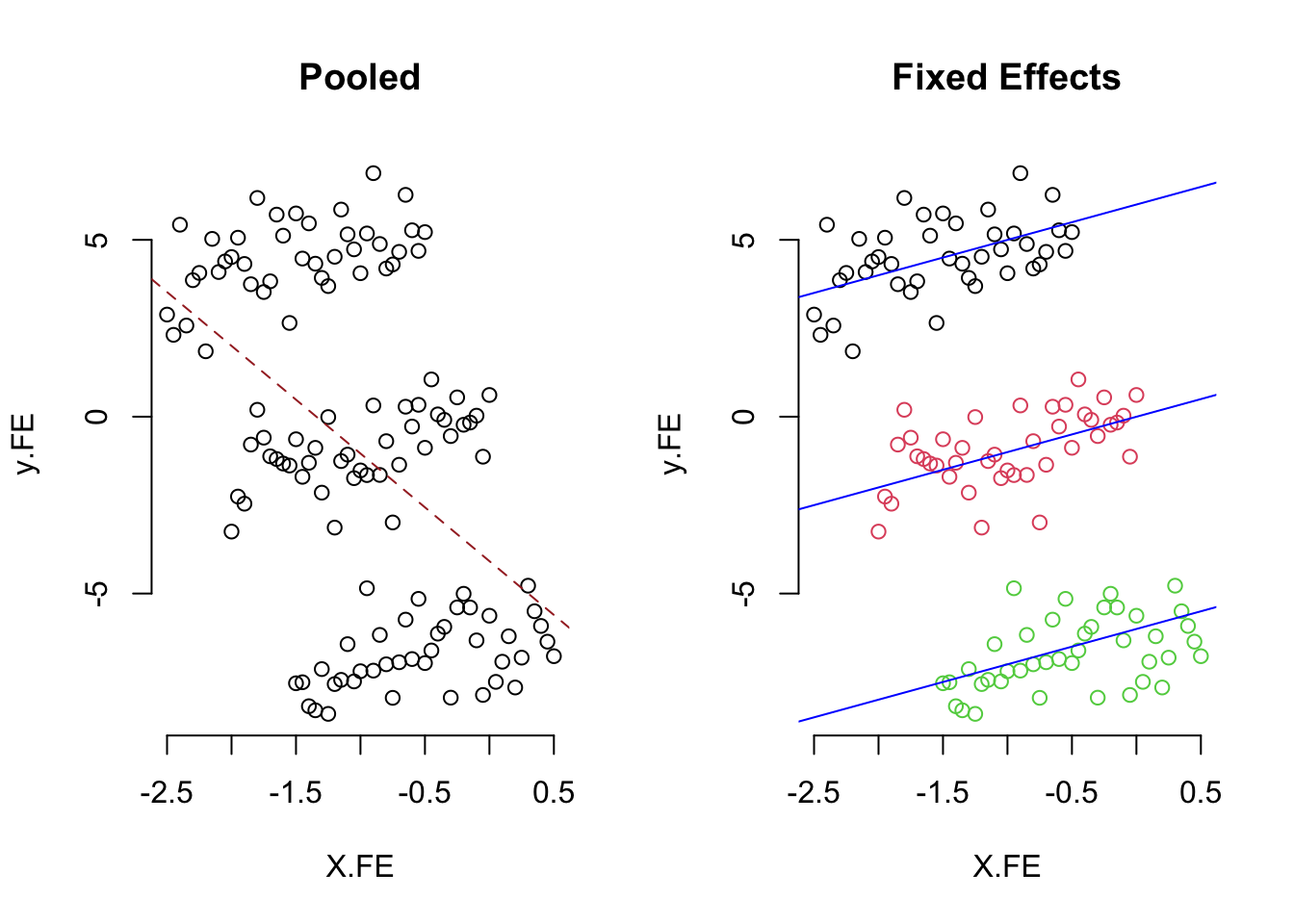
Random effects and pooled regressions can be terribly wrong when the pooled and random effects moment condition fails. Let’s show some data here to illustrate the point. The true model here is \[ y_{it} = \alpha_{i} + X_{it}\beta + \epsilon_{it} \] where the \(\beta=1\) and \(\alpha_{i}=\{6,0,-6\}\) and \(\epsilon \sim \mathcal{N}(0,1)\). Here is the plot.
The random method matters quite a bit though; many of them are very close to the truth. Models containing much or all of the between information are wrong.
If the X and unit effects are dependent, then there are serious threats to proper inference.
plm things
Beck and Katz (1995) standard errors are provided with vcovBK(). The key argument is cluster which averages over groups or time. The Beck and Katz paper would involve cluster="time".
Almost all panel unit root testing goes on with purtest. The test= argument is key for IPS, Levin, et al., Maddala-Wu, Hadri, and various tests proposed by Choi (2001). A few others are specified individually below.
The test of serial correlation for panel models is given by pbgtest(model).
The Baltagi and Li test of serial correlation in panel models with random effects is given by pbltest(model). The various alternatives are specified in alternative.
The Baltagi-Wu statistic for AR(1) disturbances is given by pbnftest(model, test="lbi") while a BNF (1982) statistic is the default for this test for fixed effects models.
# replicate Baltagi (2013), p. 101, table 5.1:
re <- plm(inv ~ value + capital, data = Grunfeld, model = "random")
pbnftest(re, test = "lbi")
pbsytest(model) gives the joint test of Baltagi and Li and a variant owing to Bera, et. al (2001) and Sosa-Escudero and Bera (2008) – the latter is a paper in Stata journal with companion software to be installed.
pcdtest(formula, data) gives the Pesaran test for cross-sectional dependence.
pdwtest(model) gives a panel Durbin-Watson statistic.
pFtest gives the F-test of fixed effects.
pggls gives GLS estimators for panel data specifying the effect and a model of within, pooling, fd.
phansitest(purtest object) combines unit root tests in the method proposed by Hanck (2013).
phtest(model1, model2) is the Hausman test for panel data models. This one has robust options detailed in the last section of ?phtest.
piest(formula, data) performs Chamberlain’s tests on the within regression.
Another test of unit/time effects is given in plmtest().
Chow tests of poolability are given by pooltest() applied to a pooled or within regression.
pvar ensures variation along dimensions.
pvcm will estimate variable coefficients models ala Swamy (1970).
Joint tests of coefficients are constructed using pwaldtest.
Wooldridge’s test for serial correlation in within models is pwartest(model)
Wooldridge’s test for AR(1) errors in level or differenced panel models is given by pwfdtest(model). The underlying idea is clever; if the levels are independent then the errors in first-differences will be correlated as -0.5. The test can be implemented against either within/fe or first-difference alternatives.
pwtest(pooling model) gives a semi-parametric test for the presence of (individual or time) unobserved effects in panel models that owes to Wooldridge.
ranef and fixef extract the random and fixed effects, respectively.